Visualizing the Dirichlet Model
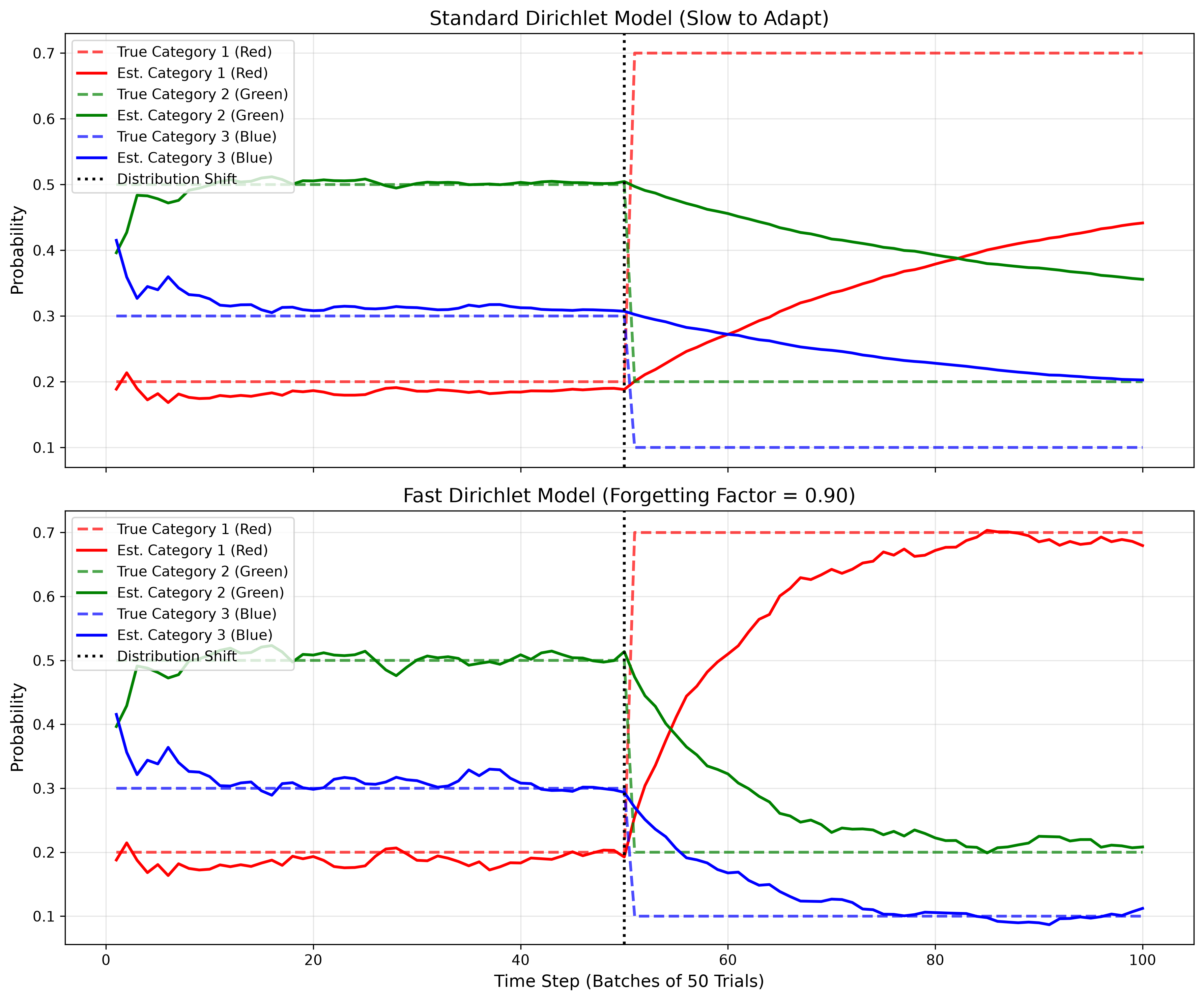
The graph below shows a 3-category system (e.g., a user choosing between Red, Green, or Blue). Initially, the true probabilities are [0.2, 0.5, 0.3]. At step 50, a UI redesign causes the probabilities to shift to [0.7, 0.2, 0.1].
Notice how the forgetting factor (\(f=0.85\)) allows the models to completely forget the old preferences and smoothly converge on the new reality.
Python Implementation (Dirichlet)
import numpy as np
import matplotlib.pyplot as plt
import os

# Ensure the images directory exists
os.makedirs('images', exist_ok=True)

class FastOnlineDirichletModel:
    def __init__(self, n_categories, alpha_prior=1.0, forgetting_factor=1.0):
        # Initialize the alpha vector with 1.0 for each category (uniform prior)
        self.alphas = np.ones(n_categories) * alpha_prior
        self.ff = forgetting_factor

    def update(self, counts_vector):
        # Apply forgetting factor to the entire alpha vector, then add new counts
        self.alphas = (self.alphas * self.ff) + counts_vector

    def get_expected_probabilities(self):
        # The expected probability for each category is alpha_i / sum(alphas)
        return self.alphas / np.sum(self.alphas)

# 1. GENERATE DATA (True probs jump at step 50)
np.random.seed(42)
n_steps = 100
n_categories = 3

# Phase 1: Red=20%, Green=50%, Blue=30%
# Phase 2: Red=70%, Green=20%, Blue=10%
data_list = []
for i in range(n_steps):
    if i < 50:
        true_probs = [0.2, 0.5, 0.3]
    else:
        true_probs = [0.7, 0.2, 0.1]

    # Simulate 10 observations per step
    counts = np.random.multinomial(10, true_probs)
    data_list.append(counts)

# 2. INITIALIZE MODELS
std_model = FastOnlineDirichletModel(n_categories, forgetting_factor=1.0)
fast_model = FastOnlineDirichletModel(n_categories, forgetting_factor=0.85)

# Lists for plotting
std_probs_history = []
fast_probs_history = []

# 3. RUN SIMULATION
for counts in data_list:
    std_model.update(counts)
    fast_model.update(counts)

    std_probs_history.append(std_model.get_expected_probabilities())
    fast_probs_history.append(fast_model.get_expected_probabilities())

# Convert to numpy arrays for easier slicing
std_probs_history = np.array(std_probs_history)
fast_probs_history = np.array(fast_probs_history)

# 4. PLOT
fig, (ax1, ax2) = plt.subplots(2, 1, figsize=(12, 10), sharex=True)

# Top plot: Standard Model (Slow)
ax1.plot(range(1, n_steps + 1), std_probs_history[:, 0], color='red', label='Category 1 (Red)')
ax1.plot(range(1, n_steps + 1), std_probs_history[:, 1], color='green', label='Category 2 (Green)')
ax1.plot(range(1, n_steps + 1), std_probs_history[:, 2], color='blue', label='Category 3 (Blue)')
ax1.axvline(x=50, color='black', linestyle='--', alpha=0.5)
ax1.set_title('Standard Dirichlet Model (Stationary Assumption)', fontsize=12)
ax1.set_ylabel('Probability')
ax1.legend(loc='upper left')
ax1.grid(True, alpha=0.3)

# Bottom plot: Fast Model (Forgetting)
ax2.plot(range(1, n_steps + 1), fast_probs_history[:, 0], color='red', label='Category 1 (Red)')
ax2.plot(range(1, n_steps + 1), fast_probs_history[:, 1], color='green', label='Category 2 (Green)')
ax2.plot(range(1, n_steps + 1), fast_probs_history[:, 2], color='blue', label='Category 3 (Blue)')
ax2.axvline(x=50, color='black', linestyle='--', alpha=0.5)
ax2.set_title('Fast Dirichlet Model (Forgetting Factor = 0.85)', fontsize=12)
ax2.set_xlabel('Time Step (Batches of 10 Trials)')
ax2.set_ylabel('Probability')
ax2.legend(loc='upper left')
ax2.grid(True, alpha=0.3)

plt.tight_layout()

# Save to the images folder
plt.savefig('images/dirichlet_graph.png', dpi=300, bbox_inches='tight')
plt.show()