5. Visualizing the Difference
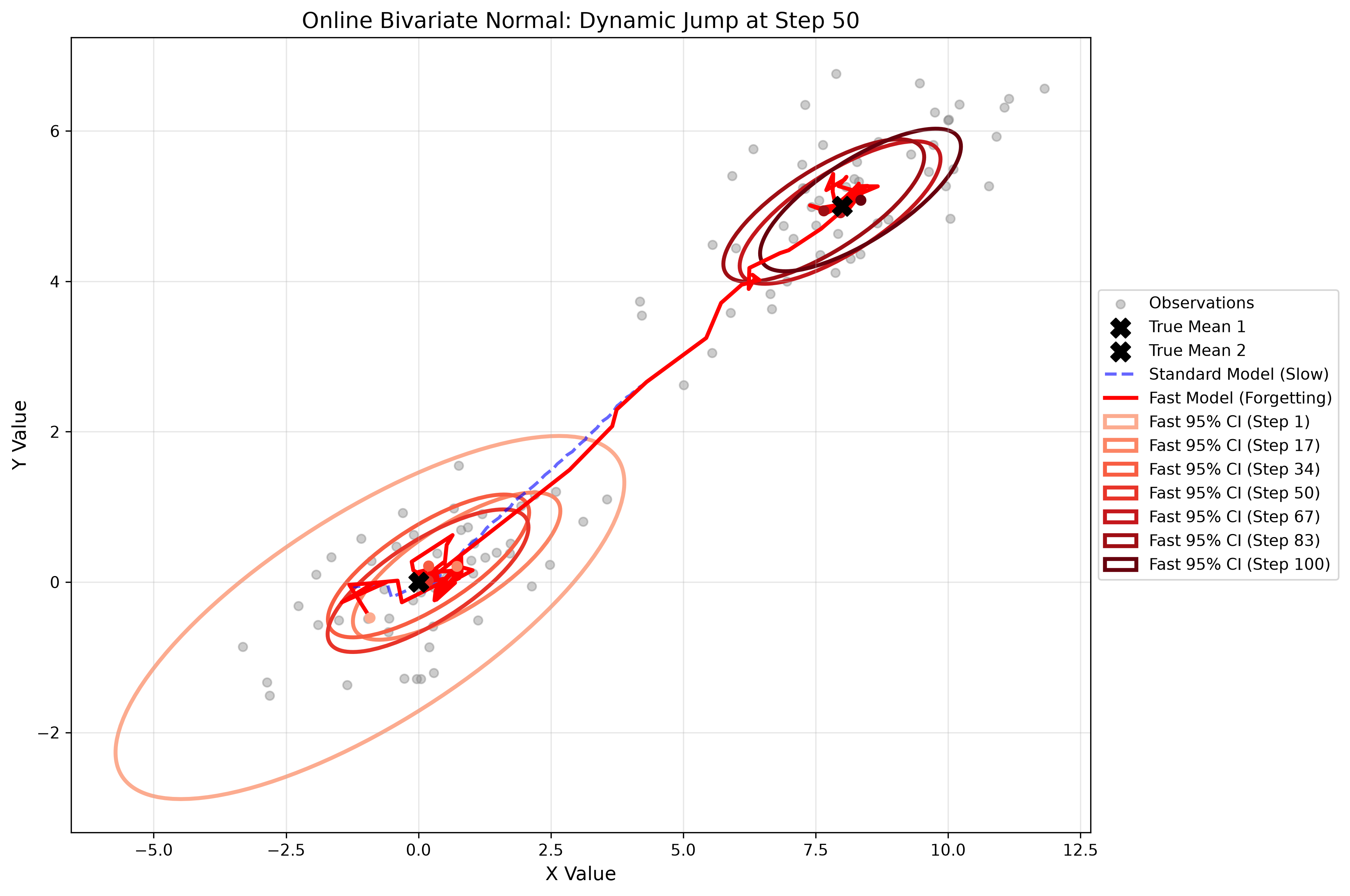
In the simulation below, a target stays at \((0,0)\) for 300 steps, then suddenly jumps to \((8,5)\).
- The Blue Dashed Line (Standard Model) is completely stuck. After 300 steps of seeing \((0,0)\), its confidence is so high that the jump to \((8,5)\) barely moves its estimate.
- The Red Line (Forgetting Model) tracks the first target, and then quickly pivots to the new target. The Red Ellipses show the 95% confidence region dynamically shifting and resizing.
Python Implementation
import numpy as np
import matplotlib.pyplot as plt
from matplotlib.patches import Ellipse
from scipy.stats import chi2
import os

# Ensure the images directory exists
os.makedirs('images', exist_ok=True)

class OnlineBivariateNormalModel:
    def __init__(self, mu_prior, cov_prior, known_cov, forgetting_factor=1.0):
        self.mu = np.array(mu_prior, dtype=float)
        self.cov = np.array(cov_prior, dtype=float)
        self.known_cov = np.array(known_cov, dtype=float)
        self.ff = forgetting_factor

    def update(self, x):
        prior_precision = np.linalg.inv(self.cov)
        data_precision = np.linalg.inv(self.known_cov)

        # Apply forgetting factor to prior precision
        discounted_precision = prior_precision * self.ff

        new_precision = discounted_precision + data_precision
        self.cov = np.linalg.inv(new_precision)
        self.mu = self.cov @ (discounted_precision @ self.mu + data_precision @ x)

    def get_ellipse_params(self, confidence=0.95):
        vals, vecs = np.linalg.eigh(self.cov)
        order = vals.argsort()[::-1]
        vals = vals[order]
        vecs = vecs[:, order]

        theta = np.degrees(np.arctan2(*vecs[:, 0][::-1]))
        chi_val = chi2.ppf(confidence, df=2)
        width, height = 2 * np.sqrt(vals * chi_val)
        return width, height, theta

# 1. GENERATE DATA (Jump happens at step 300)
np.random.seed(42)
n_steps = 600
jump_step = n_steps // 2
true_mu_1 = np.array([0, 0])
true_mu_2 = np.array([8, 5])
known_cov = np.array([[4.0, 1.5], [1.5, 1.0]])

data_list = []
for i in range(n_steps):
    if i < jump_step:
        data_list.append(np.random.multivariate_normal(true_mu_1, known_cov))
    else:
        data_list.append(np.random.multivariate_normal(true_mu_2, known_cov))

# 2. INITIALIZE MODELS
mu_prior = [0, 0]
cov_prior = [[100, 0], [0, 100]]
std_model = OnlineBivariateNormalModel(mu_prior, cov_prior, known_cov, forgetting_factor=1.0)
fast_model = OnlineBivariateNormalModel(mu_prior, cov_prior, known_cov, forgetting_factor=0.90)

std_history, fast_history = [], []
snapshot_steps = list(np.linspace(1, n_steps, num=7, dtype=int))
snapshots = []

# 3. RUN SIMULATION
for i, x in enumerate(data_list):
    std_model.update(x)
    fast_model.update(x)

    std_history.append(std_model.mu.copy())
    fast_history.append(fast_model.mu.copy())

    if (i + 1) in snapshot_steps:
        w, h, angle = fast_model.get_ellipse_params()
        snapshots.append({'step': i+1, 'mu': fast_model.mu.copy(), 'width': w, 'height': h, 'angle': angle})

# 4. PLOT
fig, ax = plt.subplots(figsize=(12, 8))
data_arr = np.array(data_list)

ax.scatter(data_arr[::5, 0], data_arr[::5, 1], color='gray', alpha=0.1, s=10, label='Observations')
ax.scatter(*true_mu_1, color='black', marker='X', s=150, zorder=5, label='True Mean 1')
ax.scatter(*true_mu_2, color='black', marker='X', s=150, zorder=5, label='True Mean 2')

std_history = np.array(std_history)
fast_history = np.array(fast_history)
ax.plot(std_history[:, 0], std_history[:, 1], 'b--', linewidth=2, alpha=0.5, label='Standard Model (Slow)')
ax.plot(fast_history[:, 0], fast_history[:, 1], 'r-', linewidth=2.5, label='Fast Model (Forgetting)')

colors = plt.cm.Reds(np.linspace(0.2, 1, len(snapshots)))
for snap, color in zip(snapshots, colors):
    ellipse = Ellipse(xy=snap['mu'], width=snap['width'], height=snap['height'],
                      angle=snap['angle'], facecolor='none', edgecolor=color,
                      linewidth=2.5, label=f"Fast 95% CI (Step {snap['step']})")
    ax.add_patch(ellipse)
    ax.plot(snap['mu'][0], snap['mu'][1], 'o', color=color, markersize=6)

ax.set_title(f'Online Bivariate Normal: Dynamic Jump at Step {jump_step}', fontsize=14)
ax.set_xlabel('X Value')
ax.set_ylabel('Y Value')
ax.grid(True, alpha=0.3)
ax.legend(loc='center left', bbox_to_anchor=(1, 0.5))
plt.tight_layout()

# Save to the images folder
plt.savefig('images/bivariate_graph.png', dpi=300, bbox_inches='tight')
plt.show()