5. Visualizing the Difference
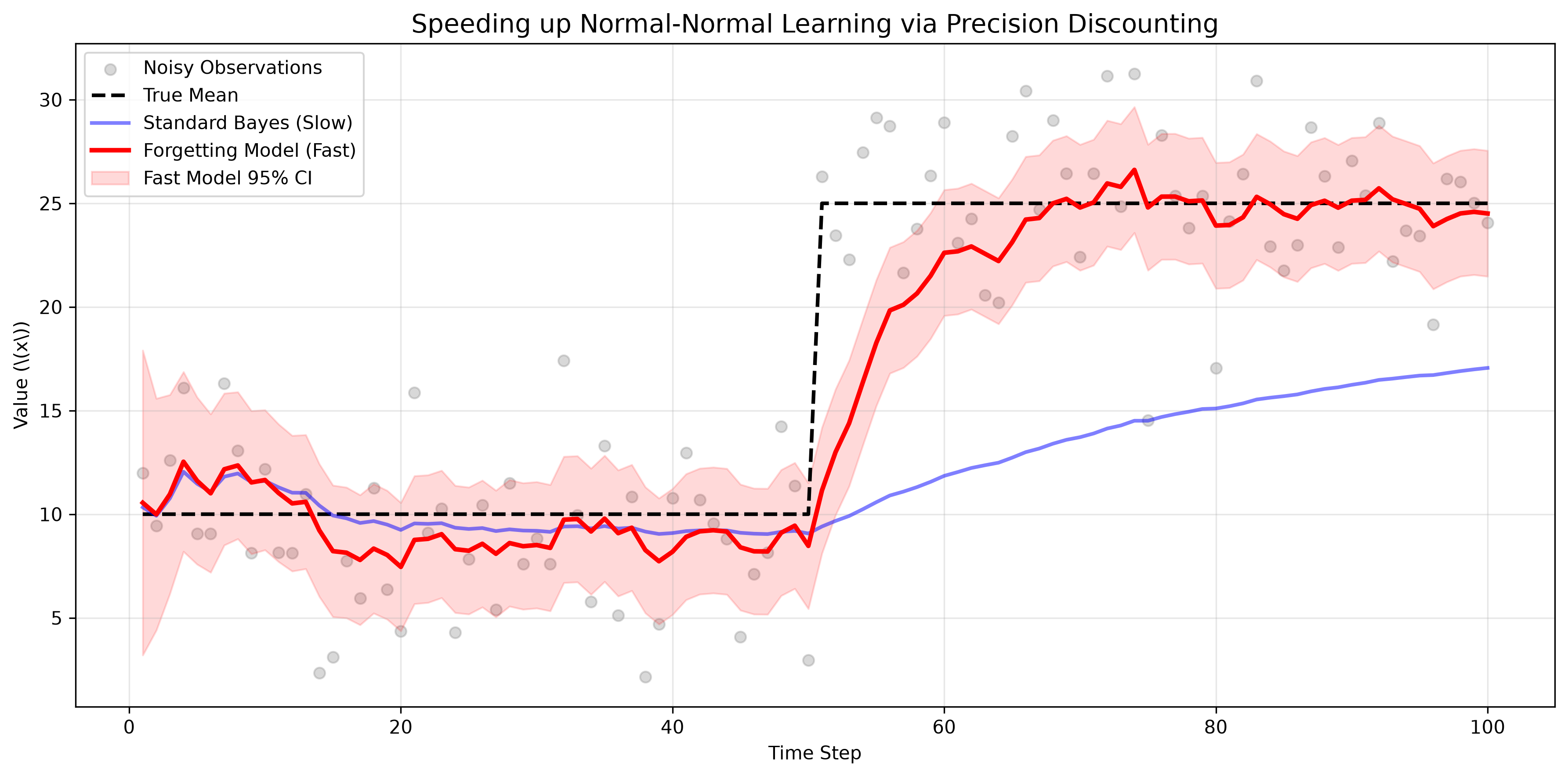
In this simulation, we take noisy sensor readings (standard deviation of 4) of a true mean that starts at 10. At step 50, the true mean abruptly jumps to 25.
Python Implementation
import numpy as np
import matplotlib.pyplot as plt
from scipy.stats import norm
import os

# Ensure the images directory exists
os.makedirs('images', exist_ok=True)

class FastOnlineNormalModel:
    def __init__(self, mu_prior=0.0, var_prior=100.0, known_var=16.0, forgetting_factor=1.0):
        self.mu = mu_prior
        self.var = var_prior
        self.known_var = known_var
        self.ff = forgetting_factor

    def update(self, x):
        # Convert variances to precisions (1/variance)
        prior_precision = 1.0 / self.var

        # Apply forgetting factor to prior precision (inflate variance)
        discounted_precision = prior_precision * self.ff
        data_precision = 1.0 / self.known_var

        # Calculate new precision and new variance
        new_precision = discounted_precision + data_precision
        self.var = 1.0 / new_precision

        # Calculate new mean
        self.mu = (discounted_precision * self.mu + data_precision * x) / new_precision

    def get_credible_interval(self, confidence=0.95):
        lp = (1.0 - confidence) / 2.0
        up = 1.0 - lp
        std_dev = np.sqrt(self.var)
        return norm.ppf(lp, loc=self.mu, scale=std_dev), norm.ppf(up, loc=self.mu, scale=std_dev)

# 1. GENERATE DATA (True mean jumps from 10 to 25 at step 50)
np.random.seed(42)
n_steps = 100
true_mu_phase1 = 10
true_mu_phase2 = 25
true_var = 16.0 # Known measurement noise (standard deviation of 4)

data_list = []
for i in range(n_steps):
    true_mu = true_mu_phase1 if i < 50 else true_mu_phase2
    data_list.append(np.random.normal(true_mu, np.sqrt(true_var)))

# 2. INITIALIZE MODELS
# Very weak prior (var=100), and we know the data variance (16)
standard_model = FastOnlineNormalModel(0, 100, true_var, forgetting_factor=1.0) # Static
fast_model = FastOnlineNormalModel(0, 100, true_var, forgetting_factor=0.85)     # Dynamic

# Lists for plotting
std_means, fast_means = [], []
fast_lb, fast_ub = [], []

# 3. RUN SIMULATION
for x in data_list:
    standard_model.update(x)
    fast_model.update(x)

    std_means.append(standard_model.mu)
    fast_means.append(fast_model.mu)

    lb, ub = fast_model.get_credible_interval()
    fast_lb.append(lb); fast_ub.append(ub)

# 4. PLOT
plt.figure(figsize=(12, 6))
plt.scatter(range(1, n_steps + 1), data_list, alpha=0.3, color='gray', label='Noisy Observations')
plt.plot(range(1, n_steps + 1), [10]*50 + [25]*50, 'k--', linewidth=2, label='True Mean')

plt.plot(range(1, n_steps + 1), std_means, 'b-', linewidth=2, alpha=0.5, label='Standard Bayes (Slow)')
plt.plot(range(1, n_steps + 1), fast_means, 'crimson', linewidth=2.5, label='Forgetting Model (Fast)')
plt.fill_between(range(1, n_steps + 1), fast_lb, fast_ub, color='crimson', alpha=0.15, label='Fast Model 95% CI')

plt.title('Speeding up Normal-Normal Learning via Precision Discounting', fontsize=14)
plt.xlabel('Time Step')
plt.ylabel(r'Value (\(x\))')
plt.legend(loc='upper left')
plt.grid(True, alpha=0.3)
plt.tight_layout()

# Save to the images folder
plt.savefig('images/normal_graph.png', dpi=300, bbox_inches='tight')
plt.show()