4. Visualizing the Difference
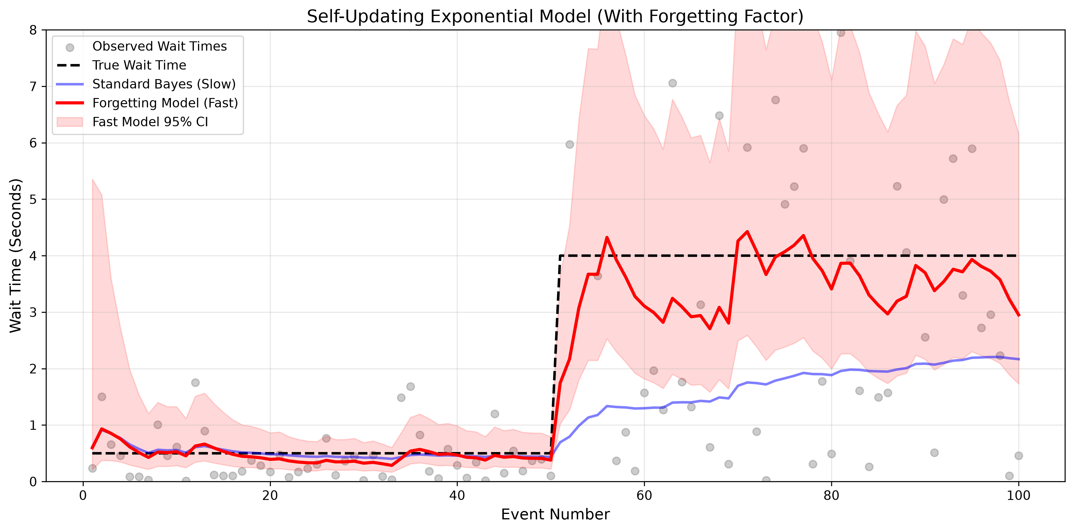
In the simulation below, a server initially processes requests with a fast wait time of 0.5 seconds (True Rate = 2.0). At event 25, the server gets overloaded and wait times jump to 4.0 seconds (True Rate = 0.25).
Python Implementation
import numpy as np
import matplotlib.pyplot as plt
from scipy.stats import gamma
import os

# Ensure the images directory exists
os.makedirs('images', exist_ok=True)

class FastOnlineExponentialModel:
    def __init__(self, alpha_prior=1.0, beta_prior=1.0, forgetting_factor=1.0):
        self.alpha = alpha_prior
        self.beta = beta_prior
        self.ff = forgetting_factor

    def update(self, wait_time):
        # Apply forgetting factor to old memory, then add new data
        self.alpha = (self.alpha * self.ff) + 1
        self.beta = (self.beta * self.ff) + wait_time

    def get_expected_wait_time(self):
        # Expected rate is alpha/beta, so wait time is beta/alpha
        return self.beta / self.alpha

    def get_credible_interval(self, confidence=0.95):
        lp = (1.0 - confidence) / 2.0
        up = 1.0 - lp
        scale = 1.0 / self.beta

        # Bounds for rate
        lb_rate = gamma.ppf(lp, a=self.alpha, scale=scale)
        ub_rate = gamma.ppf(up, a=self.alpha, scale=scale)

        # Invert bounds for wait time (note the swap)
        return 1.0 / ub_rate, 1.0 / lb_rate

# 1. GENERATE DATA (True wait jumps from 0.5s to 4.0s at step 25)
np.random.seed(42)
n_steps = 50
true_rate_phase1 = 2.0   # 0.5s wait
true_rate_phase2 = 0.25  # 4.0s wait

data_list = []
for i in range(n_steps):
    if i < 25:
        wait_time = np.random.exponential(1.0 / true_rate_phase1)
    else:
        wait_time = np.random.exponential(1.0 / true_rate_phase2)
    data_list.append(wait_time)

# 2. INITIALIZE MODELS
standard_model = FastOnlineExponentialModel(forgetting_factor=1.0) # Static
fast_model = FastOnlineExponentialModel(forgetting_factor=0.88)     # Dynamic

# Lists for plotting
std_wait_times, fast_wait_times = [], []
fast_lb, fast_ub = [], []

# 3. RUN SIMULATION
for wait_time in data_list:
    standard_model.update(wait_time)
    fast_model.update(wait_time)

    std_wait_times.append(standard_model.get_expected_wait_time())
    fast_wait_times.append(fast_model.get_expected_wait_time())

    lb, ub = fast_model.get_credible_interval()
    fast_lb.append(lb); fast_ub.append(ub)

# 4. PLOT
plt.figure(figsize=(12, 6))
plt.scatter(range(1, n_steps + 1), data_list, alpha=0.4, color='gray', label='Observed Wait Times')
plt.plot(range(1, n_steps + 1), [0.5]*25 + [4.0]*25, 'k--', linewidth=2, label='True Wait Time')

plt.plot(range(1, n_steps + 1), std_wait_times, 'b-', linewidth=2, alpha=0.5, label='Standard Bayes (Slow)')
plt.plot(range(1, n_steps + 1), fast_wait_times, 'darkorange', linewidth=2.5, label='Forgetting Model (Fast)')
plt.fill_between(range(1, n_steps + 1), fast_lb, fast_ub, color='orange', alpha=0.15, label='Fast Model 95% CI')

plt.title('Speeding up Exponential-Gamma Learning via Forgetting Factor', fontsize=14)
plt.xlabel('Event Number')
plt.ylabel('Wait Time (Seconds)')
plt.ylim(0, 8)
plt.legend(loc='upper left')
plt.grid(True, alpha=0.3)
plt.tight_layout()

# Save to the images folder
plt.savefig('images/exponential_graph.png', dpi=300, bbox_inches='tight')
plt.show()