5. Visualizing the Difference
In this simulation, an interface starts with a true success probability of 30% (meaning users typically experience 2 or 3 failures before success). At experiment 50, a new interface is introduced that is much more intuitive, jumping the success probability to 80% (users succeed almost immediately).
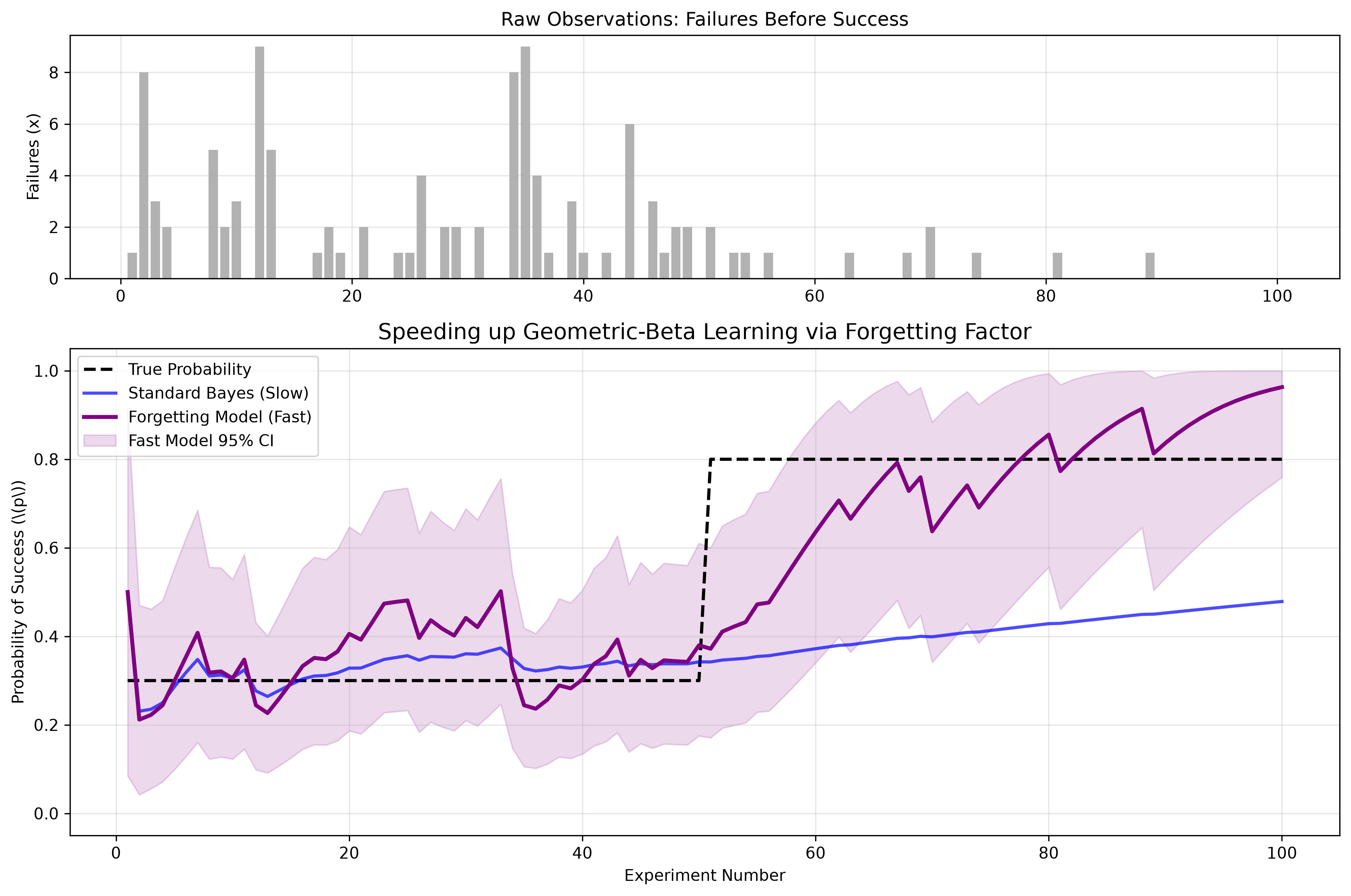
Python Implementation
import numpy as np
import matplotlib.pyplot as plt
from scipy.stats import beta
import os

# Ensure the images directory exists
os.makedirs('images', exist_ok=True)

class FastOnlineGeometricModel:
    def __init__(self, alpha_prior=1.0, beta_prior=1.0, forgetting_factor=1.0):
        self.alpha = alpha_prior
        self.beta = beta_prior
        self.ff = forgetting_factor

    def update(self, failures):
        # Apply forgetting factor to old memory, then add new data
        self.alpha = (self.alpha * self.ff) + 1
        self.beta = (self.beta * self.ff) + failures

    def get_expected_probability(self):
        return self.alpha / (self.alpha + self.beta)

    def get_credible_interval(self, confidence=0.95):
        lp = (1.0 - confidence) / 2.0
        up = 1.0 - lp
        return beta.ppf(lp, self.alpha, self.beta), beta.ppf(up, self.alpha, self.beta)

# 1. GENERATE DATA (True prob jumps from 0.3 to 0.8 at step 50)
np.random.seed(42)
n_steps = 100
true_p_phase1 = 0.3
true_p_phase2 = 0.8

data_list = []
for i in range(n_steps):
    true_p = true_p_phase1 if i < 50 else true_p_phase2
    # np.random.geometric returns total trials (k >= 1). Failures = trials - 1
    trials = np.random.geometric(true_p)
    data_list.append(trials - 1)

# 2. INITIALIZE MODELS
standard_model = FastOnlineGeometricModel(forgetting_factor=1.0) # Static
fast_model = FastOnlineGeometricModel(forgetting_factor=0.85)     # Dynamic

# Lists for plotting
std_probs, fast_probs = [], []
fast_lb, fast_ub = [], []

# 3. RUN SIMULATION
for failures in data_list:
    standard_model.update(failures)
    fast_model.update(failures)

    std_probs.append(standard_model.get_expected_probability())
    fast_probs.append(fast_model.get_expected_probability())
    lb, ub = fast_model.get_credible_interval()
    fast_lb.append(lb); fast_ub.append(ub)

# 4. PLOT
fig, (ax1, ax2) = plt.subplots(2, 1, figsize=(12, 8), gridspec_kw={'height_ratios': [1, 2]})

# Top plot: Raw Failures
ax1.bar(range(1, n_steps + 1), data_list, color='gray', alpha=0.6)
ax1.set_title('Raw Observations: Failures Before Success', fontsize=12)
ax1.set_ylabel('Failures (x)')
ax1.grid(True, alpha=0.3)

# Bottom plot: Probability tracking
ax2.plot(range(1, n_steps + 1), [0.3]*50 + [0.8]*50, 'k--', linewidth=2, label='True Probability')
ax2.plot(range(1, n_steps + 1), std_probs, 'b-', linewidth=2, alpha=0.5, label='Standard Bayes (Slow)')
ax2.plot(range(1, n_steps + 1), fast_probs, 'purple', linewidth=2.5, label='Forgetting Model (Fast)')
ax2.fill_between(range(1, n_steps + 1), fast_lb, fast_ub, color='purple', alpha=0.15, label='Fast Model 95% CI')

ax2.set_title('Speeding up Geometric-Beta Learning via Forgetting Factor', fontsize=14)
ax2.set_xlabel('Experiment Number')
ax2.set_ylabel(r'Probability of Success (\(p\))')
ax2.set_ylim(-0.05, 1.05)
ax2.legend(loc='upper left')
ax2.grid(True, alpha=0.3)

plt.tight_layout()

# Save to the images folder
plt.savefig('images/geometric_graph.png', dpi=300, bbox_inches='tight')
plt.show()