1. Introduction
In many machine learning and data science applications, we need to model the number of independent events occurring within a fixed time interval. Examples include the number of customers arriving at a store per hour, the number of server requests per second, or the number of defects on a manufacturing line. The standard statistical tool for this is the Poisson distribution.
However, in real-world scenarios, data streams are continuous, and the underlying rate of these events may change over time. A static model trained on historical data will fail to capture these shifts. This chapter explores the Poisson-Gamma conjugate Bayesian model and demonstrates how introducing an exponential forgetting factor transforms a rigid, static model into a highly adaptive, online-learning system.
2. The Standard Mathematical Setup
In Bayesian statistics, we want to estimate the unknown rate parameter \(\lambda\) (lambda), which represents the expected number of events per time interval.
The Likelihood (Poisson)
Given \(n\) observed time intervals with \(y_i\) events each, the likelihood of the data given the rate \(\lambda\) is:
\[
P(y \mid \lambda) = \prod_{i=1}^n \frac{\lambda^{y_i} e^{-\lambda}}{y_i!} \propto \lambda^{\sum y_i} e^{-n\lambda}
\]
The Prior (Gamma)
Because \(\lambda\) must be positive, we place a Gamma distribution prior on it. The Gamma distribution is the conjugate prior for the Poisson likelihood, meaning the prior and posterior share the same mathematical family. We define it with a shape parameter \(\alpha\) and a rate parameter \(\beta\):
\[
P(\lambda) = \frac{\beta^\alpha}{\Gamma(\alpha)} \lambda^{\alpha-1} e^{-\beta\lambda} \propto \lambda^{\alpha-1} e^{-\beta\lambda}
\]
The Posterior (Bayes' Theorem)
By multiplying the Likelihood and the Prior, we get the Posterior:
\[
P(\lambda \mid y) \propto \left( \lambda^{\sum y_i} e^{-n\lambda} \right) \times \left( \lambda^{\alpha-1} e^{-\beta\lambda} \right)
\]
\[
P(\lambda \mid y) \propto \lambda^{(\alpha + \sum y_i) - 1} e^{-(\beta + n)\lambda}
\]
This is exactly the form of a new Gamma distribution with updated parameters:
- \(\alpha_{\text{new}} = \alpha_{\text{prior}} + \sum y_i\) (Total events observed)
- \(\beta_{\text{new}} = \beta_{\text{prior}} + n\) (Total time intervals observed)
The Expected Rate is simply the mean of the Gamma distribution: \(E[\lambda] = \frac{\alpha}{\beta}\).
3. The Limitation: The Stationarity Assumption
The standard Bayesian update above is mathematically optimal if the world never changes. It acts as a permanent accumulator. If you have observed a rate of 5 events per hour for 1,000 hours, your parameters will be \(\alpha=5000, \beta=1000\).
If the underlying rate suddenly drops to 1 event per hour, the model will barely notice. It will take hundreds of new observations just to overcome the massive "memory" of the old data. This is because the model assumes stationarity (the statistical properties of the process do not change over time).
4. The Improvement: Exponential Forgetting
To make the model learn faster and adapt to sudden changes, we must introduce a forgetting factor (denoted as \(f\), where \(0 < f \le 1\)).
Before adding the new data, we multiply the historical parameters by \(f\). If \(f = 0.90\), the model retains 90% of its memory and loses 10% at every single step. This effectively caps the maximum "confidence" the model can achieve, allowing it to pivot when the data distribution shifts.
The Dynamic Update Rule:
\[
\alpha_{\text{new}} = (f \cdot \alpha_{\text{prior}}) + \text{observed events}
\]
\[
\beta_{\text{new}} = (f \cdot \beta_{\text{prior}}) + \text{time intervals}
\]
5. Visualizing the Difference
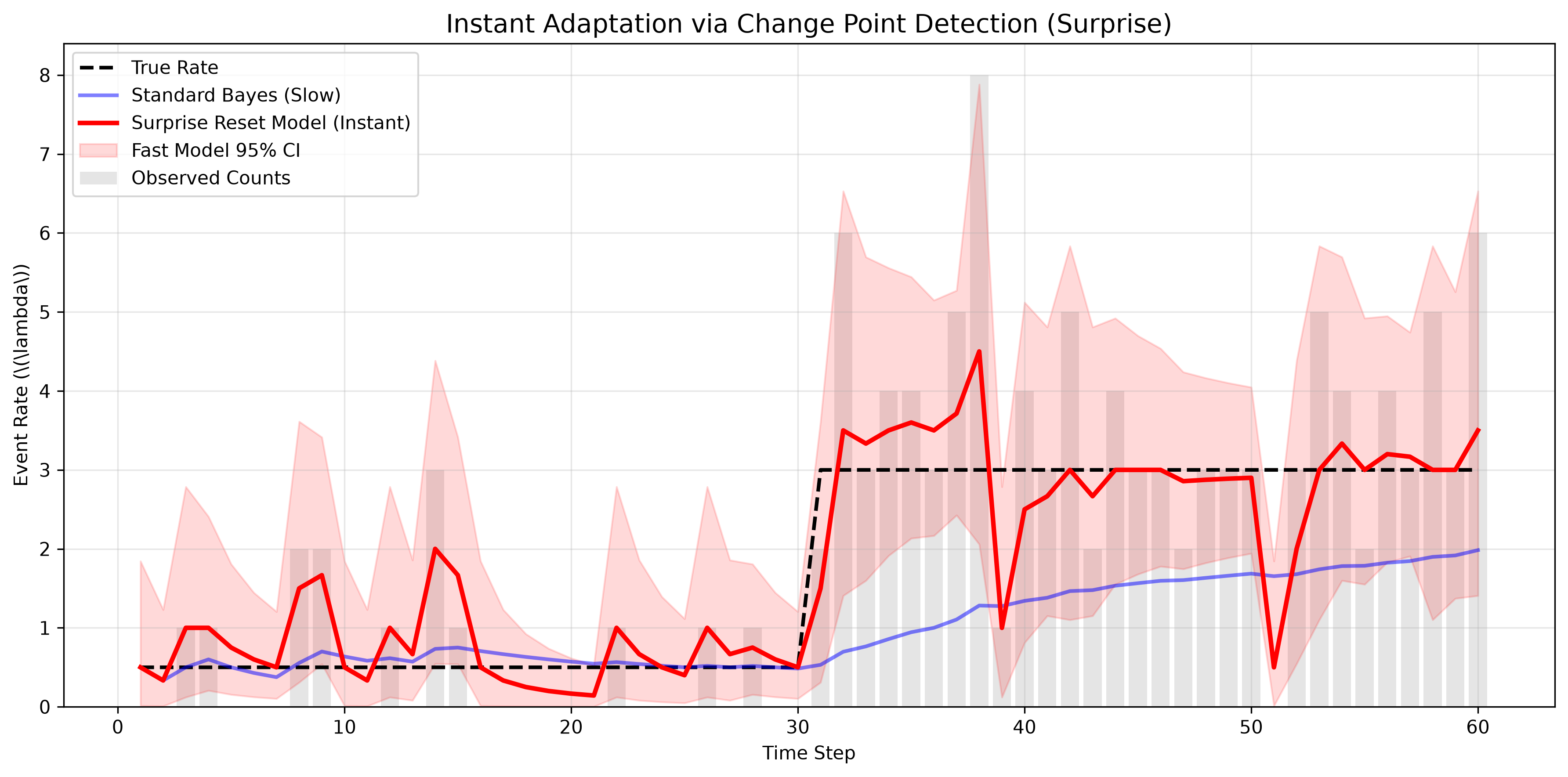
The Python script below simulates a scenario where the true event rate starts at 0.5 (Phase 1), and halfway through the simulation, jumps dramatically to 3.0 (Phase 2).
- The Blue Line represents standard Bayes. It is smooth but takes almost 20 steps to climb to the new rate after the jump.
- The Red Line represents the model with a forgetting factor of
f=0.85. It adapts to the initial rate instantly and locks onto the new rate (3.0) within just 2-3 steps after the jump.
Python Implementation
import numpy as np
import matplotlib.pyplot as plt
from scipy.stats import gamma

class FastOnlinePoissonModel:
    def __init__(self, alpha_prior=1.0, beta_prior=1.0, forgetting_factor=1.0):
        self.alpha = alpha_prior
        self.beta = beta_prior
        self.ff = forgetting_factor

    def update(self, observed_count, time_interval=1.0):
        # Apply forgetting factor to old memory, then add new data
        self.alpha = (self.alpha * self.ff) + observed_count
        self.beta = (self.beta * self.ff) + time_interval

    def get_expected_rate(self):
        return self.alpha / self.beta

    def get_credible_interval(self, confidence=0.95):
        lp = (1.0 - confidence) / 2.0
        up = 1.0 - lp
        scale = 1.0 / self.beta
        return gamma.ppf(lp, a=self.alpha, scale=scale), gamma.ppf(up, a=self.alpha, scale=scale)

# 1. GENERATE DATA (True rate starts at 0.5, jumps to 3.0 at step 30)
np.random.seed(42)
n_steps = 60
data_list = [np.random.poisson(0.5) if i < 30 else np.random.poisson(3.0) for i in range(n_steps)]

# 2. INITIALIZE MODELS
standard_model = FastOnlinePoissonModel(forgetting_factor=1.0) # No forgetting
fast_model = FastOnlinePoissonModel(forgetting_factor=0.85)     # Fast adaptation

# Lists for plotting
std_rates, fast_rates = [], []
fast_lb, fast_ub = [], []

# 3. RUN SIMULATION
for count in data_list:
    standard_model.update(count)
    fast_model.update(count)

    std_rates.append(standard_model.get_expected_rate())
    fast_rates.append(fast_model.get_expected_rate())
    lb, ub = fast_model.get_credible_interval()
    fast_lb.append(lb); fast_ub.append(ub)

# 4. PLOT
plt.figure(figsize=(12, 6))
plt.bar(range(1, n_steps + 1), data_list, alpha=0.2, color='gray', label='Observed Counts')
plt.plot(range(1, n_steps + 1), [0.5]*30 + [3.0]*30, 'k--', linewidth=2, label='True Rate')
plt.plot(range(1, n_steps + 1), std_rates, 'b-', linewidth=2, alpha=0.5, label='Standard Bayes (Slow)')
plt.plot(range(1, n_steps + 1), fast_rates, 'r-', linewidth=2.5, label='Forgetting Model (Fast)')
plt.fill_between(range(1, n_steps + 1), fast_lb, fast_ub, color='red', alpha=0.15, label='Fast Model 95% CI')

plt.title('Speeding up Poisson-Gamma Learning via Forgetting Factor', fontsize=14)
plt.xlabel('Time Step')
plt.ylabel(r'Event Rate (\(\lambda\))')
plt.legend(loc='upper left')
plt.grid(True, alpha=0.3)
plt.tight_layout()
plt.show()